Fixed-source manufactured-solution case

This page documents Morana’s fixed-source method of manufactured solutions (MMS) verification case. Its executable form is examples/fixed_source_mms.py.

At each refinement level, the case solves a three-group, nonfissioning diffusion problem with radial and axial diffusion, unequal-height layers, P0 scattering with non-unit neutron multiplicity, volumetric sources, and nonzero Dirichlet boundary data. The source, reference flux, and boundary values are evaluated independently of Morana’s assembled operators. The case also exercises balance reporting and directional excluded-region boundary selection.

Method of manufactured solutions

MMS is a code-verification technique for partial-differential-equation solvers. Choose a sufficiently smooth exact field, substitute it into the continuous equations to derive a forcing term and boundary data, then compare the discrete solution with independently evaluated exact values as the mesh is refined. It tests implementation consistency and observed accuracy; it is not experimental validation of the model. This example applies the general MMS code-verification pattern described by Salari and Knupp (2000); its geometry, fields, material data, and acceptance criteria are Morana-specific.

Target geometry and refinements

The limiting domain is the regular hexagonal prism

\[ \Omega=\operatorname{hex}(R)\times[0,H], \qquad a=60\ \mathrm{cm},\quad R=\frac{2a}{\sqrt{3}} =40\sqrt{3}\ \mathrm{cm},\quad H=108\ \mathrm{cm}, \]

where \(a\) is the planar center-to-flat distance (apothem) and \(R\) is the standard center-to-corner distance (circumradius). The planar hexagon has vertices

\[ (\pm R,0),\qquad \left(\pm\frac{R}{2},\ \pm\frac{\sqrt{3}R}{2}\right). \]

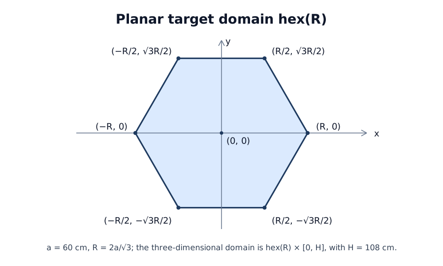
At every refinement level, the modeled active core has a complete regular hexagonal cluster as its planar cross section. The union of its control volumes converges to the target hexagonal prism as the pitch decreases. Let \(\Omega_p\) be this active planar union at pitch \(p\). For a cluster with \(n\) rings, its circumscribed large hexagon fixes the largest permitted pitch as

\[ \frac{R}{p}=n-\frac{1}{3}, \qquad p=\frac{R}{n-\frac{1}{3}}. \]

The resulting \(\Omega_p\) is wholly inside \(\operatorname{hex}(R)\), and its faceted, cell-face boundary approaches the target hexagon from the inside as \(p\) decreases. The levels do not form a nested sequence, but their boundary displacement from the target is \(O(p)\), so \(\Omega_p\) converges to \(\operatorname{hex}(R)\). The top and bottom faces are unchanged at \(z=0\) and \(z=H\).

Level	Active rings	Complete mesh rings	Pitch [cm]	Axial layers	Maximum layer height [cm]
0	3	4	25.981	6	24
1	4	5	18.895	9	16
2	6	7	12.226	12	12

The axial meshes retain unequal heights. Each of the three base bands, with heights \(2H/9\), \(3H/9\), and \(4H/9\), is split into two equal sublayers at level 0, three at level 1, and four at level 2. Both radial and axial resolution therefore increase over the study.

Each active three-dimensional control volume carries one scalar-flux unknown per energy group. With \(G=3\), active-cell counts of \(114\), \(333\), and \(1{,}092\) give \(3\times114=342\), \(3\times333=999\), and \(3\times1{,}092=3{,}276\) degrees of freedom at levels 0, 1, and 2, respectively. The count excludes the topological shell described next.

Active core and inactive shell

The example uses the material mesh itself to express local radial Dirichlet data using supported topology selectors.

Complete-mesh allocation	Key and status	Purpose
Outermost OpenMC ring (ring == 0)	A unique mms_shell_z<layer>_p<position> excluded key	Inactive shell that exposes local to_excluded radial faces
Every inner ring	Active mms_medium material	Manufactured-solution control volumes

Every shell key is registered as an ExcludedRegion of kind mms_boundary. The shell serves only as topology: a radial face of an active cell sees a known, addressable excluded neighbor. Shell cells have no cross sections, volumetric source, unknown, flux result, or balance contribution.

For each active radial face, the example assigns a unique prescribed-flux condition using both the excluded key and the direction label:

BoundaryCondition.dirichlet(face_average).on_excluded(
    key=shell_key,
    direction=face_direction,
)

For illustration, two assignments from refinement level 1 are shown below. Level 1 is the second of the three levels in the table above; it has four active rings and nine axial layers. Its zero-based axial layer 4 is the fifth layer, spanning \(36\le z\le48\ \mathrm{cm}\). Each face_average... placeholder stands for a prescribed face-average flux computed independently by quadrature.

# active_id=5, direction="u-"
BoundaryCondition.dirichlet(face_average_z4_p7_u_minus).on_excluded(
    key="mms_shell_z4_p7",
    direction="u-",
)

# active_id=14, direction="u+"
BoundaryCondition.dirichlet(face_average_z4_p19_u_plus).on_excluded(
    key="mms_shell_z4_p19",
    direction="u+",
)

An excluded shell cell can neighbor more than one active cell, but the pair (shell_key, face_direction) identifies one active face. Shell keys are also unique by axial layer, so the value may vary with axial position. The example asserts that every active radial boundary face is to_excluded, none is outer, and each resolves to its intended local Dirichlet assignment.

The following schematic uses Morana’s x, u, and v face-direction labels and its OpenMC-style orientation="x" ring-position ordering: positions start at positive x and proceed clockwise.

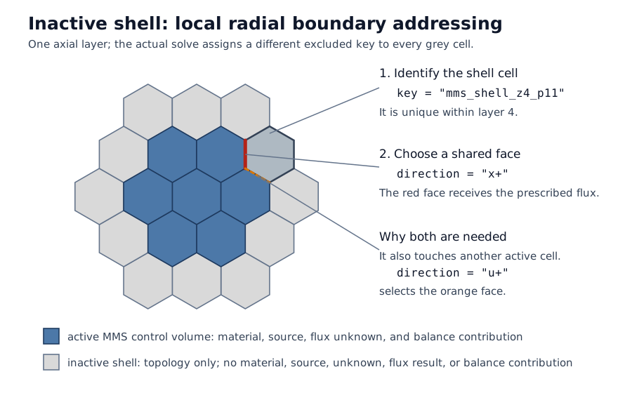
At levels 0, 1, and 2 there are respectively 30, 42, and 66 such active radial faces per layer. Multiplying by 6, 9, and 12 layers gives whole-domain totals of 180, 378, and 792.

Top and bottom are ordinary physical exterior faces. Their prescribed vectors are assigned with on_bottom() and on_top().

Exact multigroup field

Public group order is fast to thermal. Define

\[ X=\frac{\pi x}{a},\qquad Y=\frac{\pi y}{\sqrt{3}a},\qquad Z=\frac{\pi z}{H}, \]

and, for each group,

\[ f_g(x,y)=a_g\cos(X)\cos(Y)+b_g\sin(2X)\cos(Y), \]

\[ \phi_g(x,y,z)=\Phi_g[1+\sin(Z)f_g(x,y)]. \]

Group \(g\)	\(\Phi_g\) [n cm\(^{-2}\) s\(^{-1}\)]	\(a_g\)	\(b_g\)
0	\(1.20\times10^{12}\)	0.12	0.07
1	\(0.85\times10^{12}\)	-0.09	0.11
2	\(0.65\times10^{12}\)	0.08	-0.10

The coefficients keep all three exact fluxes positive while giving each a distinct shape. Since \(\sin(Z)=0\) at \(z=0\) and \(z=H\), the axial boundary data are the constant vector \((\Phi_0,\Phi_1,\Phi_2)\).

Manufactured source

The homogeneous, nonfissioning material uses

\[ D=(1.40,0.80,0.35)\ \mathrm{cm}, \]

\[ \Sigma_a=(0.030,0.040,0.055)\ \mathrm{cm}^{-1}, \]

and the complete P0 scattering matrix, indexed by incident and outgoing group, in \(\mathrm{cm}^{-1}\):

\[ \Sigma_s= \begin{bmatrix} 0.0030 & 0.0040 & 0.0010\\ 0.0005 & 0.0025 & 0.0060\\ 0.0002 & 0.0008 & 0.0040 \end{bmatrix}. \]

The matching incident-to-outgoing scattering-multiplicity matrix is

\[ M= \begin{bmatrix} 1.10 & 1.15 & 1.05\\ 1.00 & 0.90 & 1.10\\ 1.20 & 1.00 & 1.05 \end{bmatrix}. \]

There is no fission production. Ordinary scattering events define removal,

\[ \Sigma_{r,g}=\Sigma_{a,g}+ \sum_h\Sigma_{s,g\to h}-\Sigma_{s,g\to g}, \]

while scattering-neutron coupling is defined componentwise by

\[ C_{g,h} = \begin{cases} M_{g,h}\Sigma_{s,g\to h}, & g\ne h,\\ (M_{g,g}-1)\Sigma_{s,g\to g}, & g=h. \end{cases} \]

Equivalently,

\[ C=M\odot\Sigma_s- \operatorname{diag}\!\left(\operatorname{diag}\Sigma_s\right). \]

Here the nested diagonal notation extracts the diagonal of \(\Sigma_s\) and places it back on a diagonal matrix. The chosen coefficients exercise both kinds of non-unit-multiplicity effect, including signed same-group coupling. Evaluating the independently prescribed source from the exact multigroup field gives

\[ Q_g=-D_g\nabla^2\phi_g+\Sigma_{r,g}\phi_g -\sum_h C_{h,g}\phi_h. \]

The radial Laplacian is evaluated directly from

\[ \nabla_{xy}^2\bigl[\cos(X)\cos(Y)\bigr] =-\left[\left(\frac{\pi}{a}\right)^2 +\left(\frac{\pi}{\sqrt{3}a}\right)^2\right]\cos(X)\cos(Y). \]

For \(\sin(2X)\cos(Y)\), the squared \(x\) factor becomes \(\left(2\pi/a\right)^2\), while the \(y\) factor is unchanged. The axial term contributes \(-\left(\pi/H\right)^2\sin(Z)f_g\). The selected coefficients make every cell-averaged source value finite and nonnegative, as required by the fixed-source input contract. Source units are \(\mathrm{n\,cm^{-3}\,s^{-1}}\).

Discrete MMS data

The continuous manufactured fields must be reduced to one value per active hex-z control volume \(c\). The example independently computes the volume averages

\[ \bar Q_{g,c}=\frac{1}{V_c}\int_cQ_g\,dV, \qquad \bar\phi_{g,c}=\frac{1}{V_c}\int_c\phi_g\,dV. \]

\(\bar Q_{g,c}\) is the volumetric source density passed to CellSource; it has units \(\mathrm{n\,cm^{-3}\,s^{-1}}\). \(\bar\phi_{g,c}\) is the cell-average reference flux used for the error calculation and has the same meaning as Morana’s scalar-flux unknown. During finite-volume assembly, Morana multiplies the source density by the cell volume, so its volume-integrated right-hand-side contribution is \(\bar Q_{g,c}V_c\).

To calculate these integrals, the example splits each hexagon into six triangles. Each triangle is formed by the cell center \(\boldsymbol r_c\) and two consecutive vertices. Number the vertices \(\boldsymbol v_0,\ldots, \boldsymbol v_5\) counterclockwise. Then triangle \(j\) uses \(\boldsymbol v_j\) and \(\boldsymbol v_{(j+1)\bmod 6}\), with

\[ \boldsymbol a_j=\boldsymbol v_j-\boldsymbol r_c, \qquad \boldsymbol b_j=\boldsymbol v_{(j+1)\bmod 6}-\boldsymbol r_c. \]

Thus \(\boldsymbol a_j\) and \(\boldsymbol b_j\) are the vectors from \(\boldsymbol r_c\) to triangle \(j\)’s two outer vertices, and \(J_j=|\boldsymbol a_j\mathbin{\times}\boldsymbol b_j|\). The map

\[ \boldsymbol r_j(t,s)=\boldsymbol r_c+ t\bigl[(1-s)\boldsymbol a_j+s\boldsymbol b_j\bigr], \qquad z=z_0+h\zeta, \]

maps \((t,s,\zeta)\in[0,1]^3\) to triangle \(j\)’s axial prism. Its Jacobian is \(tJ_jh\). Thus, for a group component \(F\), the independently evaluated cell integral is approximated by

\[ \int_c F\,dV \approx \sum_{j=0}^{5}\sum_{i,k,\ell=1}^{3} \omega_i\omega_k\omega_\ell\, \xi_iJ_jh\, F\!\left( \boldsymbol r_j(\xi_i,\xi_k),z_0+h\xi_\ell \right). \]

Here \(\xi_i\) and \(\omega_i\) are the three-point Gauss–Legendre nodes and weights mapped from \([-1,1]\) to \([0,1]\):

\[ \boldsymbol\xi= \left(\frac{1-\sqrt{3/5}}{2},\frac12, \frac{1+\sqrt{3/5}}{2}\right), \qquad \boldsymbol\omega= \left(\frac5{18},\frac49,\frac5{18}\right). \]

The rule therefore uses \(6\times3^3=162\) quadrature points per control volume. See the NIST Digital Library of Mathematical Functions discussion of Gauss quadrature; the example obtains these nodes and weights through NumPy’s leggauss routine. This independent quadrature supplies both CellSource and the reference flux; no Morana matrix or assembled right-hand side is used to construct either value.

The radial boundary condition is imposed on the actual rectangular faces of \(\partial\Omega_p\). For every such face \(f\), the assigned Dirichlet vector is the area average

\[ \bar\phi_{g,f}=\frac{1}{A_f}\int_f\phi_g\,dA. \]

The example approximates this integral numerically. It uses the same three-point Gauss–Legendre rule as the volume average, but with two rather than three tensor-product coordinates: one along the face and one through the layer. Let \(\boldsymbol x_f\) be the face center, \(\boldsymbol\tau_f\) its unit in-plane tangent, \(\ell_f\) its length, and \(h\) the layer height. In this mapping it is convenient to retain the standard nodes and weights on \([-1,1]\),

\[ \hat{\boldsymbol\xi}=(-\sqrt{3/5},0,\sqrt{3/5}), \qquad \hat{\boldsymbol\omega}= \left(\frac59,\frac89,\frac59\right). \]

The example then evaluates the face average as

\[ \bar\phi_{g,f}\approx \frac14\sum_{i,j=1}^{3}\hat\omega_i\hat\omega_j\, \phi_g\!\left( \boldsymbol x_f+\frac{\ell_f}{2}\hat\xi_i\boldsymbol\tau_f, z_0+\frac{h}{2}(1+\hat\xi_j) \right). \]

This is a nine-point tensor-product quadrature on the rectangular face. The volume rule has \(6\times3^3\) points because it integrates both coordinates of each of the six center-to-edge triangles as well as the axial coordinate. The face rule needs only \(3^2\) points. Both evaluate the manufactured field independently of Morana’s assembled operator, so each discrete problem uses a numerical approximation to the manufactured trace on its own ragged boundary.

Morana uses this scalar face value in its documented one-sided cell-center-to-face Dirichlet elimination. The corresponding face-integrated right-hand-side contribution is \(\mathcal{G}_{g,c,f}\bar\phi_{g,f}\), with the conductance and outward-current sign convention defined in the boundary theory.

Measures and acceptance criteria

The reported solution error at refinement level \(i\) is the volume-weighted relative norm

\[ E_{2,i}= \left[ \frac{\sum_{g,c}V_{c,i}\left(\phi^{(i)}_{g,c}-\bar\phi^{(i)}_{g,c}\right)^2} {\sum_{g,c}V_{c,i}\left(\bar\phi^{(i)}_{g,c}\right)^2} \right]^{1/2}. \]

Successive observed orders use the actual planar-pitch ratio. For either error measure \(\mathcal E\in\{E_2,E_\infty\}\),

\[ q_{i\to i+1}(\mathcal E)= \frac{\log(\mathcal E_i/\mathcal E_{i+1})} {\log(p_i/p_{i+1})}. \]

Here \(i\) labels the refinement level, \(p_i\) its planar hex pitch, \(\phi^{(i)}\) the computed flux, and \(\bar\phi^{(i)}\) the independently evaluated exact cell average.

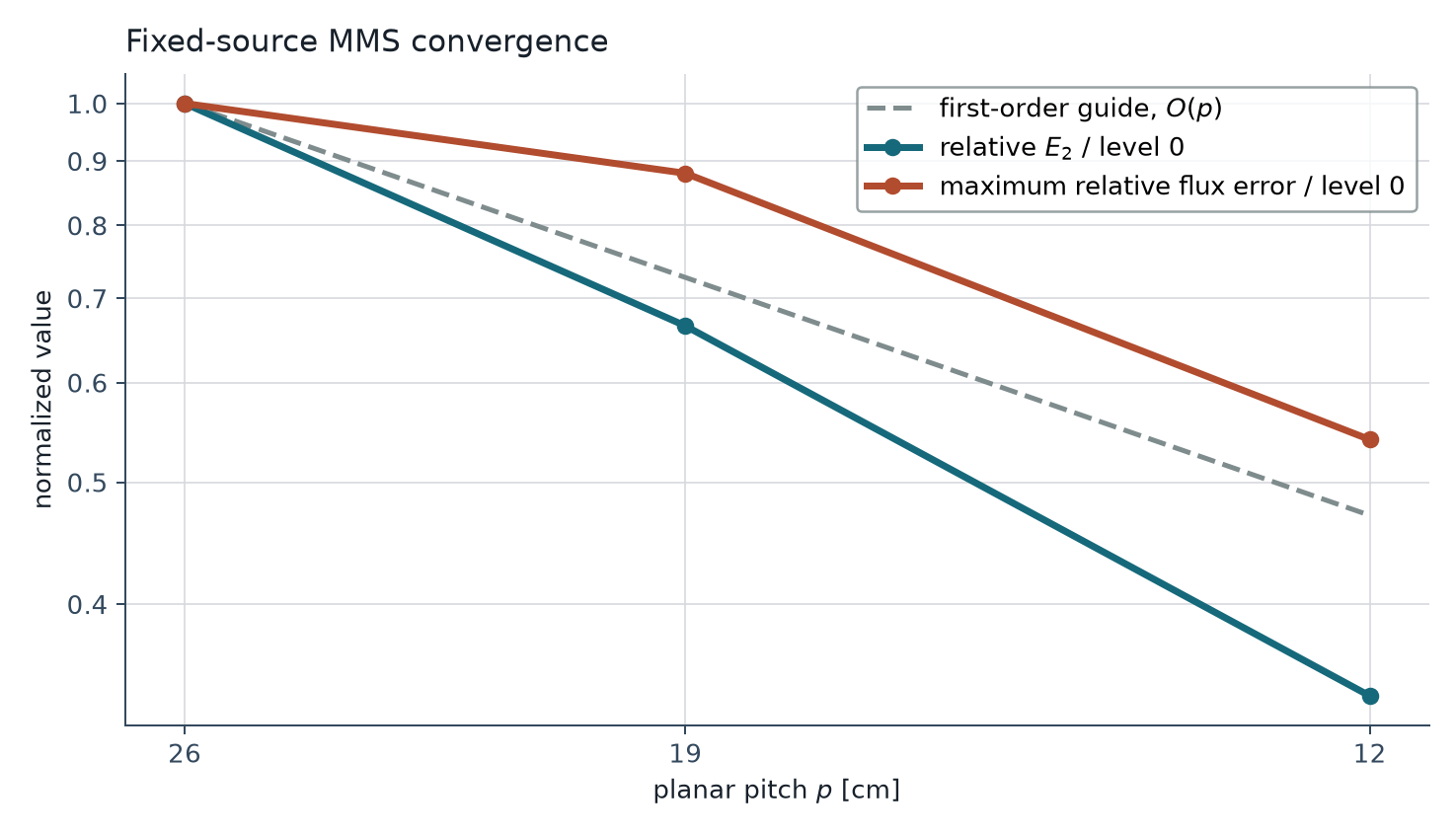
The convergence plot also tracks the maximum relative flux error over every group and active cell:

\[ E_{\infty,i}= \max_{g,c}\frac{\left|\phi^{(i)}_{g,c}-\bar\phi^{(i)}_{g,c}\right|} {\bar\phi^{(i)}_{g,c}}. \]

Both error measures are normalized to their level-0 values:

\[ \widehat E_{2,i}=\frac{E_{2,i}}{E_{2,0}}, \qquad \widehat E_{\infty,i}=\frac{E_{\infty,i}}{E_{\infty,0}}. \]

Therefore both curves begin at 1.0 at level 0 and show complementary global and worst-case solution-error behavior. The linear and scalar balance residuals are used as acceptance checks during solution.

The executable example requires all of the following:

• relative linear residual and scalar balance residual at most \(10^{-11}\);
• strictly decreasing \(E_2\) over the three levels;
• strictly decreasing \(E_\infty\) over the three levels.

Observed orders are reported as diagnostics, not acceptance thresholds. They do not by themselves establish an asymptotic order for this short, nonuniform-refinement study: each level has a different, ragged active domain whose boundary is displaced by \(O(p)\), so the domains are not nested and the set of exposed radial faces changes between levels. In addition, the supplied cell-average source, reference flux, and boundary traces are numerical Gauss–Legendre quadratures rather than analytic integrals. Their finite quadrature error contributes to the measured solution error alongside the finite-volume discretization error. Unequal axial-layer heights provide a further changing resolution scale. Establishing an asymptotic rate would require more refinement levels and a quadrature-sensitivity study.

Results and reproduction

Run the maintained case from the repository root:

python examples/fixed_source_mms.py

To repeat the full refinement study with every supported direct and GMRES linear policy, add --compare-strategies:

python examples/fixed_source_mms.py --compare-strategies

Each policy is checked independently against the manufactured flux and the same residual, balance, and refinement-error acceptance criteria. The ordinary run remains direct-only so that generating its verification figures stays compact. The option prints per-strategy/per-level error and residual rows and writes them to strategy_comparison.csv. For a one-level table that also reports informational timing and Krylov counts, run examples/solver_comparison.py.

The checked-in convergence and flux figures are regenerated from the same executable study with:

python examples/fixed_source_mms.py --documentation-assets-dir docs/assets

The recorded direct-solve results are:

Level	Relative \(E_2\)	\(E_2\) order	Maximum relative flux error	Maximum-error order
0	\(3.139\times10^{-3}\)	—	\(1.094\times10^{-2}\)	—
1	\(2.089\times10^{-3}\)	1.278	\(9.631\times10^{-3}\)	0.401
2	\(1.061\times10^{-3}\)	1.555	\(5.915\times10^{-3}\)	1.120

The largest relative linear residual is \(6.73\times10^{-16}\) and the largest relative scalar-balance residual is \(2.44\times10^{-16}\), both well below the \(10^{-11}\) acceptance threshold.

Representative fluxes

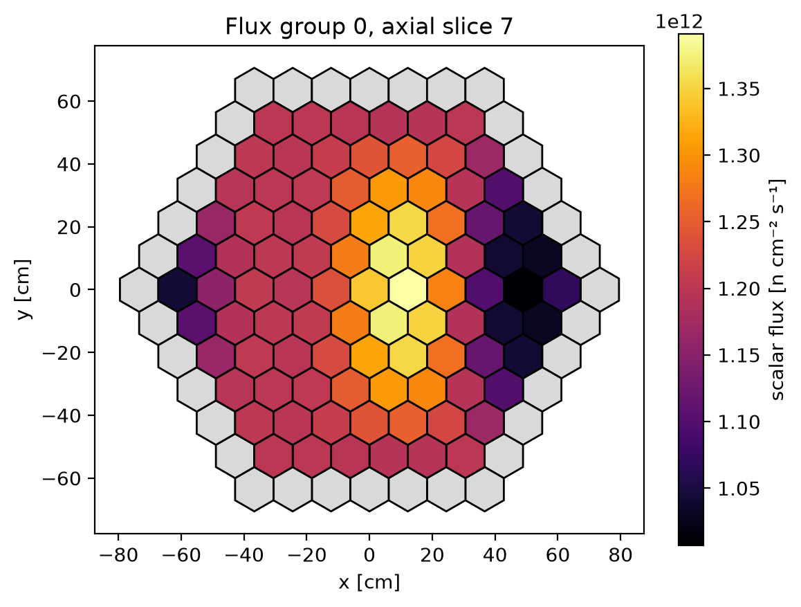
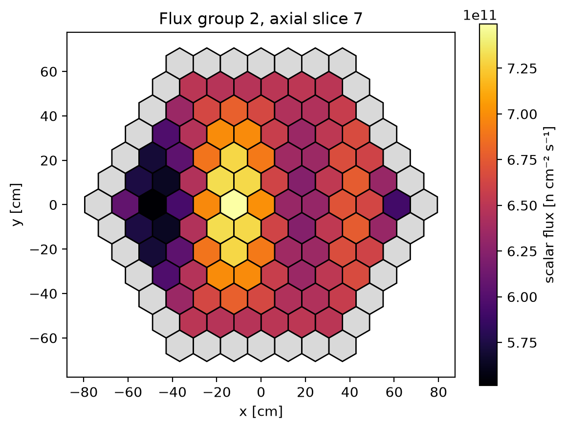
The finest mesh’s axial slice nearest the physical midplane shows the distinct fast and thermal manufactured responses. Gray cells are the inactive shell; they do not participate in the solve.

Convergence

Output artifacts

By default, the run writes convergence.csv, convergence.png, a finest-level material-layout PNG, fast and thermal midplane-flux PNGs, and a material-aware VTM file under artifacts/examples/fixed_source_mms/. The material-layout plot deliberately collapses the many uniquely keyed shell cells into one inactive shell legend entry; the shell schematic and face-resolution assertions retain their individual identities.

The CSV records pitch, maximum axial height, both solution-error measures, residuals, the whole-geometry radial-face count defined above, and observed orders for both error measures. The convergence plot uses logarithmic planar pitch \(p\) on its horizontal axis, ordered coarse to fine from left to right. Its dashed \(O(p)\) curve is a visual first-order guide anchored at the level-0 normalized value, not an acceptance threshold.

Return to the verification overview for the scope of this evidence or the maintained examples for the other runnable workflows.

References

Salari and Knupp (2000). K. Salari and P. Knupp, Code Verification by the Method of Manufactured Solutions, SAND2000-1444, Sandia National Laboratories, 2000. OSTI bibliographic record and open full text.