Geometry and indexing

Morana represents a problem in three layers of description:

1. HexPlanarMesh defines the complete regular two-dimensional hexagonal lattice.
2. MaterialSlice assigns material or excluded-region keys to positions in that lattice. Positions without an assignment are excluded.
3. MaterialMesh.stack(...) arranges one or more slices from bottom to top to form the finite hex-z solution domain.

This page defines the geometry, ordering, and face conventions shared by those objects. The modeling and solver workflow describes construction and solve behavior; inspection and output describes how these conventions appear in plots and exported files.

Morana adopts OpenMC’s ring-position convention as an indexing reference. Its geometry is defined entirely by the regular lattice and (x, u) coordinates, without an OpenMC runtime dependency. The separate OpenMC MGXS importer supplies selected material data within this Morana-owned geometry.

One regular hexagonal cell

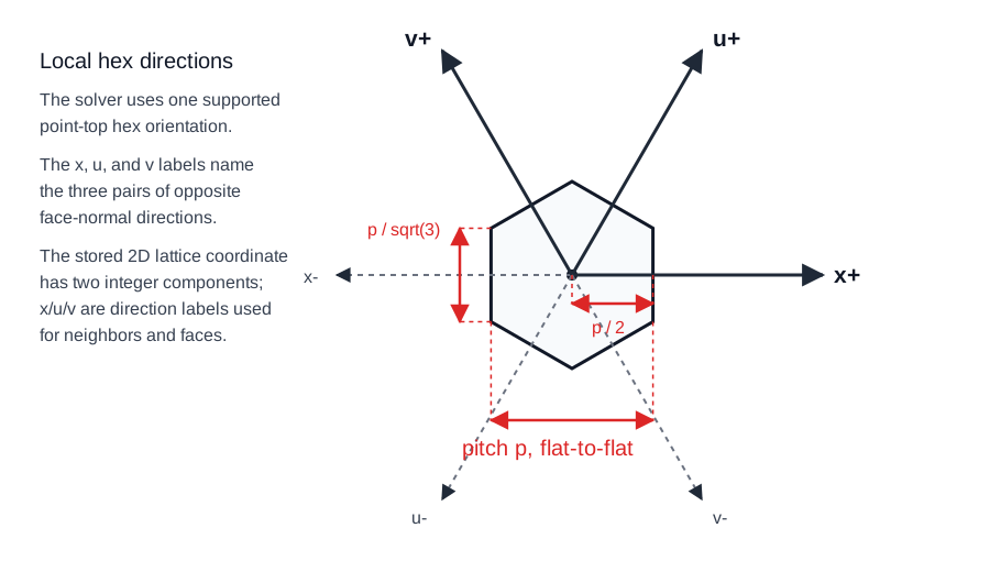
pitch is the finite positive flat-to-flat distance of a regular hexagonal cell, in cm. num_rings is a positive integer. A mesh with n = num_rings has 1 + 3 * n * (n - 1) full-lattice positions. For every cell in a regular planar mesh:

• the center-to-center distance across a shared face is pitch;
• the center-to-face distance is mesh.center_to_face == pitch / 2;
• the face length is pitch / sqrt(3);
• the cell area is sqrt(3) / 2 * pitch**2.

Morana labels the three pairs of opposite radial faces x, u, and v. The labels determine neighbor order and domain-face queries; they do not represent three stored coordinates. A lattice position has the two integer coordinates (x, u), and the third hexagonal direction is redundant.

HexPlanarMesh is immutable full-lattice geometry only: it has no material keys, active-cell IDs, or axial layers. A mesh can therefore be inspected or exported before it is overlaid by MaterialSlice and MaterialMesh. Its coords, openmc_indices, the coordinate-to-planar_id lookup, and the full-lattice neighbor table are constructed once when the mesh is created. index_of exposes that canonical coordinate lookup as an immutable mapping.

The direction names follow the established hexagonal-nodal convention shown in Figure 1 of Ferrer, Ougouag, and Bingham (2009) and Lu and Guo (2016): u and v are counterclockwise rotations of x by \(60^\circ\) and \(120^\circ\), respectively. Morana’s radial face order below remains its own API convention.

The radial face direction order is:

("x+", "x-", "u+", "u-", "v+", "v-")

Locate a planar lattice position

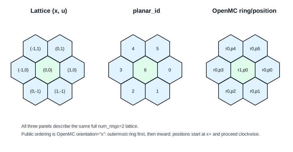
HexPlanarMesh provides three complementary identifiers for a position in its full lattice:

Identifier	Purpose
planar_id	Flattened full-lattice position used by planar-mesh inspection and geometry export.
Lattice coordinate (x, u)	Integer geometric coordinate used for topology and Cartesian cell centers.
OpenMCIndex(ring, position)	Serialized ring-position identity used for OpenMC-style input and output.

The following convention matters when reading or writing OpenMC-style ring data. Morana uses the OpenMC orientation="x" convention only. In the flattened full-lattice order, rings run from outermost to innermost. Positions within a ring start in the positive x direction and proceed clockwise. Thus a full num_rings=2 mesh has its center at planar_id = 6; a full num_rings=3 mesh has its center at planar_id = 18. Convert an OpenMC orientation="y" layout before constructing a Morana mesh.

OpenMCIndex is an immutable, hashable (ring, position) value object used as the key for sparse MaterialSlice input. Its natural ordering is lexicographic (ring, position): this follows the outer-to-inner serialized ring sequence, not a spatial walk around the entire lattice. It is a mesh-relative identifier. Construction requires non-Boolean, nonnegative integer fields, but only a HexPlanarMesh can determine whether the resulting ring-position pair belongs to that mesh. For a mesh with n rings, membership requires:

0 <= ring < n
0 <= position < max(6 * (n - 1 - ring), 1)

mesh.openmc_indices supplies the complete valid sequence. Use mesh.planar_id_at(index) for a safe reverse lookup—returning None for an out-of-mesh index—while sparse MaterialSlice construction rejects an out-of-mesh key. OpenMCIndex identifies a full planar position only; it is not the layer-dependent solver active_id.

OpenMC defines orientation in its HexLattice API and documents the associated skewed bases in its hexagonal-lattice indexing method.

Cartesian cell centers follow directly from (x, u) and the flat-to-flat pitch:

x_cart = pitch * (x + 0.5 * u)
y_cart = sqrt(3) / 2 * pitch * u

The lookup methods preserve the same full-lattice convention:

• lattice_coord(planar_id) and openmc_index(planar_id) return the two identities at a known planar position;
• planar_id_at(OpenMCIndex(ring, position)) performs the reverse lookup and returns None when that ring-position does not belong to the mesh; and
• neighbors(planar_id) returns six entries in radial direction order. An entry is another full-lattice planar_id or None at the physical planar perimeter. It does not classify material or excluded-domain interfaces.

All forward planar-ID lookups (lattice_coord, openmc_index, neighbors, cartesian_center, and cell_vertices) require a non-Boolean integer in 0 <= planar_id < n_cells. They raise TypeError for another input type and IndexError when the ID is outside the complete lattice; in particular, negative IDs never use Python’s sequence-indexing convention.

See inspection and output for full-lattice plotting and VTU export artifacts.

Select the active planar domain

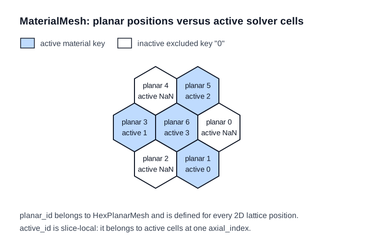
HexPlanarMesh always describes every position in the regular lattice. MaterialSlice supplies a sparse mapping from OpenMCIndex values to material keys for one layer. When slices are stacked, unassigned positions receive the built-in excluded key "0" and are inactive. A MaterialMesh can also define additional mesh-local excluded-region keys with ExcludedRegion. This lets boundary conditions distinguish holes or omitted regions without treating them as active materials.

Pass additional excluded regions when stacking. Their keys and region kinds are human-readable identifiers: each must contain a non-whitespace character and only printable characters, while preserving its exact spelling. Their values must be ExcludedRegion objects, and the built-in inactive key "0" is reserved:

material_mesh = MaterialMesh.stack(
    (lower_slice, upper_slice),
    excluded_regions={"gap": ExcludedRegion(kind="void", color="#d9d9d9")},
)

Here, "gap" is the excluded-region identity and "void" is its kind. Every "gap" position is excluded from the active solver domain, has no material cross sections or source, and can be selected with on_excluded(key="gap"). A key can occur at several positions or in disconnected regions; it does not identify a single connected component. A kind groups keys with shared semantics: for example, "beam_port_a" and "beam_port_b" can both have kind "source_port", allowing one boundary rule to select both by kind or only one by key. Keys and kinds match by exact equality. ExcludedRegion values are immutable descriptions.

The built-in "0" identity is always the reserved "inactive" kind and uses the plotting color "white". A custom region without a color uses the default excluded-region plotting color #d9d9d9. Any supplied custom color is passed through without validation and is used by layout plotting.

The two IDs serve different purposes:

• planar_id identifies a location in the complete two-dimensional lattice. It is independent of axial layer, so the same planar position has the same planar_id in every layer.
• active_id identifies an active solver cell within one selected axial layer. It skips excluded positions and may therefore differ between layers. The unique active material-mesh position is (axial_index, active_id).

Flux arrays use this compact, active-domain-only active_id order. See inspection and output for how plots and exports present those values on the complete lattice.

For a selected layer, active_indices(axial_index) returns the active positions as the subset of mesh.openmc_indices in its documented flattened order. Every layer-aware cell query takes axial_index first, followed by the local identifier: key_at(axial_index, openmc_index), active_id_at(axial_index, openmc_index), openmc_index_for_active_id(axial_index, active_id), and face(axial_index, active_id, direction). Thus the layer is selected before the planar or compact-cell position. active_id_at() returns the corresponding compact ID or None when the position is excluded or outside the full mesh; use key_at() when those cases need to be distinguished. material_by_active_id() and openmc_index_for_active_id() provide the inverse material and position views.

Stack layers in the axial direction

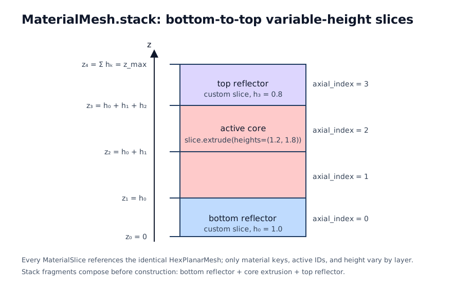
A MaterialSlice is immutable reusable planar input: one HexPlanarMesh reference, a sparse OpenMC-index material-key mapping, and one finite positive height. Direct construction is the sparse form: mapping keys must belong to the mesh, values must be strings, and the mapping is copied to a read-only view. Positions omitted from the mapping receive the inactive key "0" when the slice is stacked:

slice_0 = MaterialSlice(
    mesh,
    {OpenMCIndex(1, 0): "fuel"},
    height=2.0,
)

MaterialSlice.from_openmc_rings(mesh, rings, height=...) is the complete form. It requires one list for each mesh ring, ordered outermost to innermost, with max(6 * radius, 1) entries for a ring of radius radius. Positions in each list use the documented OpenMC orientation="x" order. Use direct construction when omitted positions should remain inactive; use ring input when the full layer layout is available.

slice.extrude(count=N) returns a bottom-to-top tuple that repeats the same immutable slice N times. slice.extrude(heights=(h_0, ...)) returns one otherwise identical slice per specified finite positive height. Provide exactly one form; both fragments can be concatenated before stacking:

slices = reflector.extrude(count=2) + core.extrude(heights=(1.2, 1.8))
material_mesh = MaterialMesh.stack(slices)

Create every material mesh, including a one-layer mesh, with MaterialMesh.stack((slice_0, ...)). Its tuple is ordered bottom to top, and all slices must reference the identical planar mesh instance.

Stacking resolves the independent layer mappings and derives the immutable axial_layer_heights tuple. Every layer-specific MaterialMesh query takes an explicit, nonnegative in-stack axial_index.

Layer numbering is bottom-up:

• axial_index = 0 is the bottom layer;
• axial_index = 1 is the layer immediately above it;
• n_axial_layers is the number of material layers.

The stack starts at z_min = 0.0 and ends at z_max, the sum of its layer heights. For h_k = axial_layer_heights[k], layer k spans:

z_min = sum(h_l for l in range(k))
z_max = z_min + h_k

Each layer repeats the same full planar lattice, but material keys, active/excluded status, compact active_id values, and face classifications are evaluated per layer. Fixed-source and k_eff solves therefore support different active-cell counts in different layers.

Faces and geometric measures

Every active hex-z cell has six radial faces and two axial faces, bottom and top. A radial neighbor is the adjoining planar lattice position in the same layer. An axial neighbor occupies the same OpenMCIndex in the layer below or above.

A face is classified as:

• internal when its neighboring position is active;
• to_excluded when its neighboring in-stack position is excluded;
• outer when it lies on the physical perimeter of the complete stack.

MaterialMesh.face() returns the resulting DomainFace topology. Its directions are x+, x-, u+, u-, v+, v-, bottom, and top. An internal face has a complete active-neighbor identity; an excluded interface has a neighboring axial/OpenMC position and excluded key/kind but no active ID; an outer face has no neighbor fields. Obtain these values from face() rather than constructing them directly.

For a layer of height h_k, a radial face has area face_length * h_k and an axial face has the planar hex-cell area. The cell volume is area * h_k. These measures, including unequal layer heights at axial interfaces, enter the finite-volume diffusion resistance; see the theory and numerical conventions for the equations.

References

Ferrer, Ougouag, and Bingham (2009). R. M. Ferrer, A. M. Ougouag, and A. A. Bingham, Nodal Green’s Function Method Singular Source Term and Burnable Poison Treatment in Hexagonal Geometry, INL/EXT-09-16773, Idaho National Laboratory, 2009. OSTI bibliographic record and open full text.

Lu and Guo (2016). D. Lu and C. Guo, “Development and Validation of a Three-Dimensional Diffusion Code Based on a High Order Nodal Expansion Method for Hexagonal-z Geometry,” Science and Technology of Nuclear Installations, 2016, Article ID 6340652, DOI 10.1155/2016/6340652. Open full text.