Theory and numerical conventions

This page is the implementation-level mathematical reference for Morana’s steady-state, multigroup neutron-diffusion solver. It defines the equations, discretization, boundary reductions, linear and eigenvalue iteration, normalizations, and residuals used by the finite-volume implementation. The cited sources provide the broader reactor-diffusion background; the modeling and solver workflow provides the input and API context. The verification guide records the evidence for these equations and their implementation.

Scope and sources

The classical diffusion, multigroup, partial-current, and criticality background follows Bell and Glasstone (1970, Chs. 2–4, especially §§2.5d, 3.1e, and 4.3–4.4). The control-volume terminology and conservative two-point flux construction follow Eymard, Gallouët, and Herbin (2000, §§1, 9.1, and 11.1). Citations identify the background result being used. Array ordering, geometric packing, the affine boundary convention, the zero-diffusion limit, convergence measures, and physical normalization are Morana-specific choices defined on this page. The boundary guide defines face selection and supported condition inputs; result layouts and callable behavior are defined in the modeling and solver workflow.

Governing equation and units

The implemented finite-volume reference solver uses diffusion on a regular hex-z mesh. With no fission production and either no scattering or unit-multiplicity self-scattering, its one-group fixed-source equation reduces to

\[ -\nabla \cdot (D\nabla\phi) + \Sigma_a\phi = Q. \]

The finite-volume unknown is a cell-average scalar flux, and the matrix equation is volume-integrated. Length is expressed in cm and time in seconds: macroscopic cross sections are in \(\mathrm{cm}^{-1}\), diffusion coefficients in cm, scalar flux in \(\mathrm{n\,cm^{-2}\,s^{-1}}\), and volumetric sources in \(\mathrm{n\,cm^{-3}\,s^{-1}}\). When supplied, kappa_sigma_f is a recoverable-energy production cross section in \(\mathrm{eV\,cm^{-1}}\). Morana converts its energy factor using the exact SI relation \(1\ \mathrm{eV}=1.602176634\times10^{-19}\ \mathrm{J}\) before comparing it with a power-normalization target in W. Energy groups are ordered fast to thermal but have no stored energy bounds; temperature is not an input to the solver.

Imported diffusion coefficients

Morana normally receives each group diffusion coefficient \(D_g\) directly. The OpenMC MGXS adapter instead requires the caller to select one of two conversions from a supported runtime-library record. The "total" convention uses the runtime field exactly as stored:

\[ D_g=\frac{1}{3\Sigma_{\mathrm{stored},g}}. \]

The OpenMC XSdata.set_total_mgxs(...) API accepts either TotalXS or TransportXS for the same XSdata total cross section, which the runtime format exports as total without recording which one supplied it. Thus this conversion is uncorrected when \(\Sigma_{\mathrm{stored}}\) is a total cross section and already transport corrected when it is a transport cross section. Morana cannot infer or retain that provenance.

The "p1-outscatter" convention requires \(\Sigma_{\mathrm{stored}}=\Sigma_t\) from an uncorrected TotalXS. It uses the ordinary-event P1 scattering matrix in Morana’s incoming-to-outgoing orientation:

\[ \Sigma_{tr,g}=\Sigma_{t,g}-\sum_h\Sigma_{s1,g\to h}, \qquad D_g=\frac{1}{3\Sigma_{tr,g}}. \]

The sum fixes the incident group \(g\) and ranges over outgoing groups \(h\). This is the group-discrete form of the outscatter approximation in Ványi et al. (2021), §2.1, not the in-scatter correction used by OpenMC TransportXS and Boyd et al. (2019), Eqs. 10–11. Scattering multiplicity does not enter this correction. Applying it to a stored TransportXS would double-correct the cross section and is invalid; Morana cannot detect that provenance error from the runtime file. The importer rejects a nonfinite or nonpositive required stored or derived cross section but does not substitute another convention. OpenMC’s XSdata reference defines the source fields and array shapes.

Multigroup formulation

The implemented solver supports any positive number of energy groups across a variable-height axial stack.

Ordering and assembly

Public group-indexed data are ordered fast to thermal. Layered source and result arrays are group-major with shape (G, N), while material transfer matrices use (g_from, g_to). Global finite-volume operators use node-major, group-fastest packing, I(n, g) = nG + g, where \(n\) is a packed active-node index.

Scattering, fission, and operator split

Primitive P0 scattering data use sigma_s[g_from, g_to]: the first index is the group in which an event occurs and the second is its destination group. The scattering-neutron multiplicity matrix \(M\) has the same orientation. When every event emits one neutron, every entry of \(M\) equals one. Scattering multiplicity represents neutron-producing scattering reactions, such as \((n,xn)\) reactions. In the multigroup convention used here, each entry is the scattering-neutron production rate divided by the corresponding ordinary scattering-event rate (Boyd et al., 2019, §III.D). For one material and cell, let \(S\) be the ordinary scattering-event matrix and \(M\) the scattering-neutron multiplicity matrix. Their elementwise product \(T=M\odot S\) is the scattering-neutron transfer matrix. Morana then defines the signed scattering-coupling matrix \(C\) by

\[ C_{g,h}=\begin{cases} T_{g,h}, & g\ne h,\\ T_{g,g}-S_{g,g}, & g=h. \end{cases} \]

Classical multigroup diffusion distinguishes ordinary scattering-event removal from intergroup scattering source (Bell and Glasstone, 1970, §4.3). Morana extends that scattering treatment with signed scattering-neutron coupling to represent non-unit scattering multiplicity (Boyd et al., 2019, §III.D).

The diagonal correction subtracts the ordinary self-scattering event, so unit-multiplicity self-scattering has no net effect. Thus \(C_{g,h}\) is the signed scattering-neutron coupling from incident group \(g\) to outgoing group \(h\): off-diagonal entries are neutron emission, whereas a diagonal entry is the neutron gain or loss relative to conventional self-scattering. The \(T\) and \(C\) construction, its same-group diagonal correction, and the assembled-loss acceptance condition are Morana-specific conventions. Conventional removal remains based on ordinary event loss, not neutron emission multiplicity:

\[ \Sigma_{r,g}=\Sigma_{a,g}+\sum_{h\ne g}\Sigma_{s0,g\to h}. \]

With this incoming-to-outgoing storage, scattering coupling into group \(g\) is \(\sum_h C_{h,g}\phi_h\). Let \(H\) be the volume-integrated matrix containing conventional removal, radial and axial diffusion, and boundary loss. Let \(\mathcal{C}\) be the volume-integrated, cell-local assembly of \(C\). The public loss matrix is

\[ A=H-\mathcal{C}^T. \]

Thus the event-oriented input entry sigma_s[g_from, g_to] contributes to the assembled operator row for g_to and column for g_from; equivalently, the energy-space scattering production operator uses the transpose of the input indexing.

Its diagonal includes the volume-integrated \(-C_{g,g}\) contribution, so same-group multiplication is explicit. Unit multiplicity gives a zero coupling diagonal and recovers the ordinary-scattering operator. A steady solve requires every assembled loss diagonal to remain positive after this term and all leakage contributions are included. Consequently, nonnegative scattering multiplicities are valid input data, but loss assembly rejects a configuration whose same-group scattering multiplication makes an assembled diagonal nonpositive. Such an operator lies outside Morana’s accepted steady-solve domain.

For a one-group material, there is no intergroup scattering, but that does not make arbitrary self-scattering disappear. The formulas reduce to

\[ \Sigma_r=\Sigma_a, \qquad C_{1,1}=(M_{1,1}-1)\Sigma_{s0,1\to1}. \]

Self-scattering therefore cancels only when its multiplicity is one (or its cross section is zero). A non-unit same-group multiplicity remains a signed neutron gain or loss in the assembled equation.

Morana represents local fission neutron production with the nonnegative, event-oriented fission-transfer matrix \(T^{\mathrm{f}}\). Its entry \(T^{\mathrm{f}}_{g_{\mathrm{from}},g_{\mathrm{to}},n}\) is the production cross section from incident group \(g_{\mathrm{from}}\) to emitted group \(g_{\mathrm{to}}\) at node \(n\). This is the extracted form of fission_transfer[g_from, g_to]; its first index selects the fissioning incident group and its second selects the emitted group.

Group-to-group fission-production matrices retain both incident and emitted energy-group dependence (Boyd et al., 2019, §III.G). The incident-group fission-production cross section is the transfer row sum,

\[ p_{g,n}=\sum_h T^{\mathrm{f}}_{g,h,n}. \]

The volume-integrated fission-emission matrix is

\[ F_{(n,g_{\mathrm{to}}),(n,g_{\mathrm{from}})} =T^{\mathrm{f}}_{g_{\mathrm{from}},g_{\mathrm{to}},n}V_n. \]

Each node contributes one such \(G\times G\) block. Its rows select the group receiving fission emission and its columns select the group producing it. The separable representation is the special case

\[ T^{\mathrm{f}}_{g_{\mathrm{from}},g_{\mathrm{to}},n} =\nu\Sigma_{f,g_{\mathrm{from}},n}\chi_{g_{\mathrm{to}},n}, \]

where the normalized outgoing spectrum \(\chi\) is independent of the incident group. It gives an outer-product local block. General transfer data need not be separable and do not contain an independent \(\chi\).

The groupwise fission source functionals used throughout this page are

\[ \begin{aligned} P_g(\boldsymbol\phi) &=\sum_n p_{g,n}V_n\phi_{g,n} &&\text{(production by group $g$)}, \\ E_g(\boldsymbol\phi) &=\sum_{n,h}T^{\mathrm{f}}_{h,g,n}V_n\phi_{h,n} &&\text{(emission into group $g$)}, \\ K_g(\boldsymbol\phi,k_{\mathrm{eff}}) &=\frac{E_g(\boldsymbol\phi)}{k_{\mathrm{eff}}} &&\text{(eigenvalue-scaled source into group $g$)}. \end{aligned} \]

Because \(p_{g,n}\) is the transfer row sum,

\[ P(\boldsymbol\phi) \equiv\sum_gP_g(\boldsymbol\phi) =\sum_gE_g(\boldsymbol\phi), \qquad \sum_gK_g(\boldsymbol\phi,k_{\mathrm{eff}}) =\frac{P(\boldsymbol\phi)}{k_{\mathrm{eff}}}. \]

Fixed-source and eigenvalue systems

Let \(\mathbf b_Q\) denote the volume-integrated independent volumetric source and let \(\mathbf b_\partial\) denote all additive boundary contributions from prescribed face flux or incident partial current. Define the complete fixed-source right-hand side once as

\[ \mathbf b \equiv \mathbf b_Q+\mathbf b_\partial. \]

The canonical fixed-source problem is then

\[ \left(A-F\right)\boldsymbol\phi=\mathbf b. \]

Criticality uses the same assembled loss matrix but no independent source, giving the standard multigroup diffusion \(k\)-eigenvalue problem (Bell and Glasstone, 1970, §4.4):

\[ A\boldsymbol\phi =\frac{1}{k_{\mathrm{eff}}}F\boldsymbol\phi. \]

Finite-volume discretization

The cell-centered finite-volume scheme assembles every energy group over the complete axial material stack into one coupled sparse system. The following sections define the entries of \(H\), \(\mathbf b_Q\), and \(\mathbf b_\partial\) and apply the scattering-coupling and fission-emission operators \(\mathcal{C}\) and \(F\) to the cell balances.

A geometric active cell is \(c=(m,k)\), where \(m\) is its full-lattice planar_id and \(k\) is its axial_index. The same \(m\) denotes the same planar position in every layer, whereas active_id is slice-local and can differ between layers. The packed-node index \(n(c)\) appears only in assembled vectors and matrices.

Let the cell have volume \(V_c\), group-\(g\) cell-average flux \(\phi_{g,c}\), diffusion coefficient \(D_{g,c}\), derived removal cross section \(\Sigma_{r,g,c}\), and volumetric source \(Q_{g,c}\). Integrating the fixed-source group equation over \(c\) gives the local conservative balance that defines the finite-volume method (Eymard, Gallouët, and Herbin, 2000, §1, Example 1.2, Eq. 1.8):

\[ \sum_{f\in\partial c} J_{\mathrm{out},g,c,f} A_f + \Sigma_{r,g,c}V_c\phi_{g,c} - \sum_h C_{h,g,c}V_c\phi_{h,c} - \sum_h T^{\mathrm{f}}_{h,g,c}V_c\phi_{h,c} = Q_{g,c}V_c. \]

\(J_{\mathrm{out},g,c,f}\) is positive when group-\(g\) neutrons leave cell \(c\) through face \(f\). The scattering sum is the net scattering contribution into group \(g\): it includes transfers from every other group and any same-group neutron gain or loss. It uses the local \(C_{h,g,c}\) data assembled into \(\mathcal{C}\). With unit multiplicity, \(C_{g,g,c}=0\) and \(C_{h,g,c}=\Sigma_{s0,h\to g,c}\) for \(h\ne g\), recovering the usual off-diagonal ordinary-scattering source. The fission sum is the emission into group \(g\) from every incident group; it uses the local \(T^{\mathrm{f}}_{h,g,c}\) data assembled into \(F\). For the criticality equation, \(Q_{g,c}=0\) and the fission term is divided by \(k_{\mathrm{eff}}\).

For a layer of height \(h_k\) and regular flat-to-flat hex pitch \(p\), let \(A_{\mathrm{hex}}\) be the planar hex area. The cell and face measures are

\[ \begin{aligned} A_{\mathrm{hex}} &= \frac{\sqrt{3}}{2}p^2, \\ V_c &= A_{\mathrm{hex}}h_k && \text{for $c=(m,k)$}, \\ A_{r,k} &= \frac{p}{\sqrt{3}}h_k, \\ \ell &= p && \text{(center-to-center distance)}, \\ d &= \frac{p}{2} && \text{(center-to-face distance)}. \end{aligned} \]

An internal face joins two active cells and contributes a conservative two-cell coupling. An exposed face has no active neighbor; it contributes a one-cell boundary term after its condition has been resolved. The internal radial and axial couplings are derived first, followed by the common exposed-face boundary treatment. This is a cell-centered two-point flux approximation on an orthogonal mesh. The face conductance is obtained by adding the two center-to-face diffusion resistances (Eymard, Gallouët, and Herbin, 2000, §9.1, Eq. 9.6, and §11.1, Eq. 11.4).

Radial internal faces

For each group, consider a radial internal face \(f\) shared by cells \(c=(m,k)\) and \(c'=(m',k)\). Its area is \(A_f=A_{r,k}\), and the material interface is halfway between their centers. Assuming a constant current through the two half-cell segments, their diffusion resistances add:

\[ R_{g,c,f}=\frac{\ell/2}{D_{g,c}A_f}, \qquad R_{g,c',f}=\frac{\ell/2}{D_{g,c'}A_f}. \]

The outward current integrated over the face is therefore

\[ \begin{aligned} J_{g,c\rightarrow c'}A_f &= \frac{\phi_{g,c}-\phi_{g,c'}} {R_{g,c,f}+R_{g,c',f}} \\ &= \mathcal{G}^{\mathrm{rad}}_{g,c,c'}(\phi_{g,c}-\phi_{g,c'}), \\ \mathcal{G}^{\mathrm{rad}}_{g,c,c'} &= \frac{D_{g,f}A_f}{\ell}, \\ D_{g,f} &= \frac{2D_{g,c}D_{g,c'}} {D_{g,c}+D_{g,c'}}. \end{aligned} \]

Thus \(D_{g,f}\) is the harmonic mean of the two group-specific cell diffusion coefficients. This choice preserves current continuity at a discontinuous material interface and gives the same conductance in both directions. If either cell has \(D=0\), Morana defines the harmonic mean and face conductance as zero.

Axial internal faces

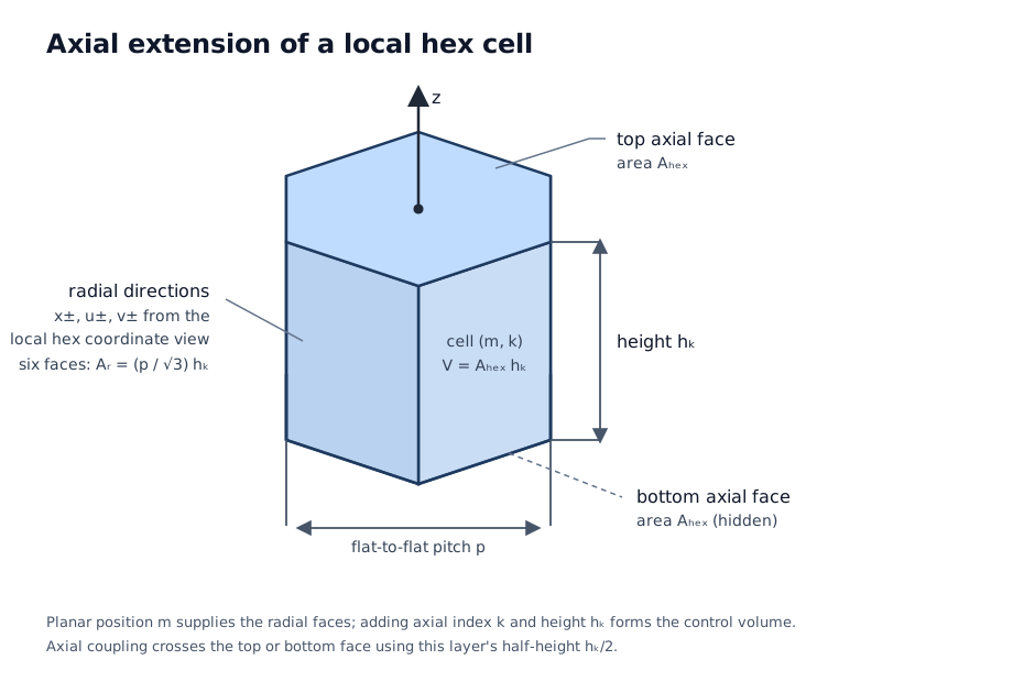
For an axial internal face \(f\), let \(c_-=(m,k)\) be the lower cell and \(c_+=(m,k+1)\) the upper cell. The face area is \(A_f=A_{\mathrm{hex}}\). The material interface need not be midway between the centers because the layer heights can differ. The two half-cell resistances and resulting conductance are, independently for each group,

\[ \begin{aligned} R^{\mathrm{ax}}_{g,c_-,f} &= \frac{h_k}{2D_{g,c_-}A_{\mathrm{hex}}}, \\ R^{\mathrm{ax}}_{g,c_+,f} &= \frac{h_{k+1}}{2D_{g,c_+}A_{\mathrm{hex}}}, \\ J_{g,c_-\rightarrow c_+}A_{\mathrm{hex}} &= \frac{\phi_{g,c_-}-\phi_{g,c_+}} {R^{\mathrm{ax}}_{g,c_-,f}+R^{\mathrm{ax}}_{g,c_+,f}} \\ &=\mathcal{G}^{\mathrm{ax}}_{g,c_-,c_+} (\phi_{g,c_-}-\phi_{g,c_+}), \\ \mathcal{G}^{\mathrm{ax}}_{g,c_-,c_+} &= \frac{A_{\mathrm{hex}}} {h_k/(2D_{g,c_-}) + h_{k+1}/(2D_{g,c_+})}. \end{aligned} \]

For the two rows associated with any internal face, let \(\mathcal{G}\) denote the applicable radial or axial conductance. Its contribution to \(H\) is

\[ H_{\mathrm{face},g}= \begin{bmatrix} \mathcal{G} & -\mathcal{G} \\ -\mathcal{G} & \mathcal{G} \end{bmatrix}. \]

It is symmetric, has zero row sum, and transfers neutrons between cells without creating or destroying them. As for radial interfaces, either adjacent cell having \(D=0\) makes the axial conductance zero.

Diffusion/removal matrix and assembled loss matrix

Let \(\mathcal{N}(c)\) be the active neighbors of cell \(c\), and let \(\mathcal{B}(c)\) be its exposed faces. Let \(\mathcal{G}_{g,c,c'}\) denote the applicable radial or axial internal-face conductance and \(\mathcal{G}_{g,c,f}\) the group-\(g\) boundary conductance derived in the next section. The assembled row of \(H\) is

\[ \begin{aligned} H_{(n(c),g),(n(c),g)} &= \Sigma_{r,g,c}V_c + \sum_{c'\in\mathcal{N}(c)}\mathcal{G}_{g,c,c'} + \sum_{f\in\mathcal{B}(c)}\mathcal{G}_{g,c,f}, \\ H_{(n(c),g),(n(c'),g)} &= \begin{cases} -\mathcal{G}_{g,c,c'}, & c'\in\mathcal{N}(c), \\ 0, & \text{otherwise}. \end{cases} \end{aligned} \]

The assembled loss matrix returned by the public assembly helper is \(A=H-\mathcal{C}^T\). The local contribution of \(-\mathcal{C}^T\) at every group pair is \(-C_{h,g,c}V_c\) in row \((n(c),g)\) and column \((n(c),h)\), including \(h=g\). In the canonical right-hand side defined above, the row entries are

\[ \begin{aligned} (b_Q)_{n(c),g} &=Q_{g,c}V_c, \\ (b_\partial)_{n(c),g} &=\sum_{f\in\mathcal{B}(c)}b_{\partial,g,c,f}, \end{aligned} \]

where \(b_{\partial,g,c,f}\) is the additive contribution from one exposed face. It is zero for homogeneous conditions, \(\mathcal{G}_{g,c,f}\phi_{b,g,f}\) for prescribed Dirichlet flux, and the affine incoming-current term derived in the next section for a boundary with imposed incidence.

Conventional removal contributes \(\Sigma_{r,g,c}V_c\) to each same-group diagonal before scattering coupling is subtracted; the fission-emission matrix supplies the remaining within-cell coupling. Each internal face contributes one symmetric two-cell block for each group, while each exposed face contributes only to its owning group row. This is a volume-integrated operator: matrix entries have units \(\mathrm{cm}^2\), flux has units \(\mathrm{n\,cm^{-2}\,s^{-1}}\), and both sides of the equation have units \(\mathrm{n\,s^{-1}}\).

Exposed boundary conditions

An exposed face has no active neighboring cell. It can be a lateral exterior face, a physical bottom or top face, or a face bordering a to_excluded material-mesh region. Let \(c=(m,k)\) be the owning geometric cell and \(f\) one of its exposed faces. The group-\(g\) physical face flux is \(\phi_{b,g,f}\), and \(D_{g,c}\) is the adjacent cell coefficient. A radial exposed face has \(A_f=A_{r,k}\) and \(d_{c,f}=p/2\); an axial exposed face has \(A_f=A_{\mathrm{hex}}\) and \(d_{c,f}=h_k/2\). Linear variation between the cell center and face gives

\[ J_{\mathrm{out},g,c,f} =D_{g,c}\frac{\phi_{g,c}-\phi_{b,g,f}}{d_{c,f}}. \]

Each remaining boundary derivation applies independently to one fixed group and one exposed pair \((c,f)\). To keep the scalar formulas readable, the fixed group index is suppressed below: \(\phi_c\) denotes \(\phi_{g,c}\) and \(D_c\) denotes \(D_{g,c}\). The local face subscripts are also suppressed on face values and distances, so \(\phi_b\) denotes \(\phi_{b,g,f}\) and \(d\) denotes \(d_{c,f}\); a conductance written \(\mathcal{G}_{cf}\) denotes \(\mathcal{G}_{g,c,f}\).

Robin and partial-current-return coefficients are scalar and apply independently to every group; prescribed flux and current spectra are group-resolved. Group-coupled boundary-response matrices are outside this model.

Bell and Glasstone (1970, §§2.5d and 3.1e) provide the physical diffusion basis for the reflective and Marshak-vacuum conditions below. Morana adopts the outward-current sign convention used on this page and derives each condition’s one-cell finite-volume contribution. The Dirichlet, generalized Robin, and partial-current-return forms below are Morana parameterizations built from standard boundary concepts.

Each exposed face must have a boundary condition. Internal active-to-active faces instead use the two-cell diffusion coupling derived above. A single finite-height layer reduces to a two-dimensional diffusion model only when zero axial current is imposed on its bottom and top faces.

Boundary-region selection is defined in boundary conditions and face selection. This section concerns the face equations after selection and covers their finite-volume reduction.

The reductions derived below can be summarized as follows. Each \(\mathcal{G}_{cf}\) contributes to the owning diagonal of \(H\), and each \(b_{\partial,cf}\) contributes to the boundary right-hand side.

Boundary condition	Face relation	\(\mathcal{G}_{cf}\)	\(b_{\partial,cf}\)
Reflective	\(J_{\mathrm{out}}=0\)	\(0\)	\(0\)
Dirichlet	\(\phi_b\) prescribed	\(D_cA_f/d\)	\(\mathcal{G}_{cf}\phi_b\)
Marshak vacuum	\(J_{\mathrm{out}}=\phi_b/2\)	\(D_cA_f/(d+2D_c)\)	\(0\)
Affine Robin	\(J_{\mathrm{out}}=\alpha\phi_b-s\)	\(\alpha D_cA_f/(D_c+\alpha d)\)	\(sD_cA_f/(D_c+\alpha d)\)

Reflective

A reflective face imposes zero normal current:

\[ J_{\mathrm{out}}=0. \]

Therefore \(\mathcal{G}_{cf}=0\); the face contributes nothing to either the matrix or right-hand side.

Dirichlet

A Dirichlet face prescribes the physical face flux \(\phi_b\). Substitution into the one-sided current approximation gives

\[ J_{\mathrm{out}}A_f = \frac{D_cA_f}{d}(\phi_c-\phi_b). \]

Defining

\[ \mathcal{G}_{cf}=\frac{D_cA_f}{d}, \]

the face adds \(+\mathcal{G}_{cf}\) to \(H_{cc}\) and \(+\mathcal{G}_{cf}\phi_b\) to \((b_\partial)_c\). A zero-Dirichlet condition therefore has no right-hand-side term and generally leaks more strongly than the vacuum approximation below. A nonzero value represents a prescribed physical face-flux field and is primarily useful for verification, truncated-domain calculations, and potential model coupling. This is a general prescribed-value boundary condition; its physical face-flux interpretation and finite-volume reduction are defined here for Morana.

Marshak vacuum

A transport vacuum means zero incoming angular flux. Diffusion theory cannot represent the angular condition directly, so it is approximated here by the Marshak condition described through diffusion-theory partial currents by Bell and Glasstone (1970, §§2.5d and 3.1e):

\[ J_{\mathrm{out}}=\frac{\phi_b}{2}, \]

equivalently

\[ \phi_b+2D_c\frac{\partial\phi}{\partial n}=0. \]

Combining this condition with the center-to-face current approximation gives

\[ \begin{aligned} D_c\frac{\phi_c-\phi_b}{d} &= \frac{\phi_b}{2}, \\ \phi_b &= \frac{2D_c}{d+2D_c}\phi_c, \\ J_{\mathrm{out}} &= \frac{D_c}{d+2D_c}\phi_c. \end{aligned} \]

The resulting face conductance is

\[ \mathcal{G}_{cf}=\frac{D_cA_f}{d+2D_c}. \]

It adds \(+\mathcal{G}_{cf}\) to \(H_{cc}\) and no right-hand-side term. The physical-face flux is nonzero; the diffusion solution extrapolates toward zero outside the physical domain.

Robin current and partial-current return

Morana parameterizes homogeneous current-to-flux boundary response with the Robin family

\[ J_{\mathrm{out}}=\alpha\phi_b, \]

where the normal points outward from the modeled domain and \(\alpha\) is the dimensionless net-current-over-face-flux coefficient. This family includes the standard reflective and Marshak-vacuum limits; the allowed range and the conductance reduction below are Morana conventions. Combining this with the one-sided finite-volume current approximation gives

\[ \begin{aligned} D_c\frac{\phi_c-\phi_b}{d} &= \alpha\phi_b, \\ \phi_b &= \frac{D_c}{D_c+\alpha d}\phi_c, \\ J_{\mathrm{out}} &= \frac{\alpha D_c}{D_c+\alpha d}\phi_c. \end{aligned} \]

The integrated face conductance is therefore

\[ \mathcal{G}_{cf}=\frac{\alpha D_cA_f}{D_c+\alpha d}. \]

This expression includes reflective boundaries at \(\alpha=0\), Marshak vacuum at \(\alpha=1/2\), and approaches zero-flux Dirichlet as \(\alpha\rightarrow\infty\). Values \(0\leq\alpha\leq1/2\) describe passive reflector-to-vacuum behavior. Larger nonnegative values are mathematical sinks and do not represent physical albedo.

For physical albedo, let \(\mu=\boldsymbol\Omega\mathbin{\cdot}\mathbf n\), where \(\mathbf n\) is the outward face normal, and choose the local \(x\) axis to point along \(\mathbf n\). The unnumbered P1 truncation of Eq. 2.57 displayed on p. 99 of Bell and Glasstone (1970, §2.5d) uses the scalar flux \(\phi_0\) and first angular moment \(\phi_1\). At the face, these are \(\phi_0=\phi_b\) and \(\phi_1=J_{\mathrm{out}}\), so in Morana’s notation it becomes

\[ \psi_{P1}(\boldsymbol\Omega) =\frac{1}{4\pi}\left(\phi_b+3\mu J_{\mathrm{out}}\right). \]

Define the nonnegative outgoing and incoming partial currents by the half-range angular integrals

\[ j^+=\int_{\mu>0}\mu\psi_{P1}(\boldsymbol\Omega)\,d\boldsymbol\Omega, \qquad j^-=-\int_{\mu<0}\mu\psi_{P1}(\boldsymbol\Omega)\,d\boldsymbol\Omega. \]

Evaluating the azimuthal integral and the remaining integrals over \(0<\mu<1\) gives

\[ j^+=\frac{\phi_b}{4}+\frac{J_{\mathrm{out}}}{2}, \qquad j^-=\frac{\phi_b}{4}-\frac{J_{\mathrm{out}}}{2}. \]

Thus

\[ j^+ + j^-=\frac{\phi_b}{2}, \qquad j^+ - j^-=J_{\mathrm{out}}. \]

Morana parameterizes scalar return using the ratio

\[ j^-=\beta j^+, \qquad 0\leq\beta\leq1. \]

Substituting this relation into the partial-current definitions gives the face flux and net outward current in terms of the outgoing partial current:

\[ \begin{aligned} \frac{\phi_b}{2} &= j^+ + j^- = j^+ + \beta j^+ = (1+\beta)j^+, \\ J_{\mathrm{out}} &= j^+ - j^- = j^+ - \beta j^+ = (1-\beta)j^+. \end{aligned} \]

Eliminating \(j^+\) yields the homogeneous Robin form

\[ J_{\mathrm{out}} =\frac{1-\beta}{2(1+\beta)}\phi_b =\alpha\phi_b. \]

Consequently,

\[ \alpha=\frac{1-\beta}{2(1+\beta)}, \qquad \beta=\frac{1-2\alpha}{1+2\alpha}. \]

Thus \(\beta=1\) gives perfect return and \(\alpha=0\), while \(\beta=0\) gives the Marshak-vacuum response and \(\alpha=1/2\). In Morana’s convention, \(\beta\) is the returned-to-outgoing partial-current ratio, whereas \(\alpha\) is the net-outward-current-to-face-flux ratio.

An independent nonnegative incident partial current can be included as

\[ j^-=\beta j^+ + q_{\mathrm{in}}, \]

where \(q_{\mathrm{in}}\) is the surface-averaged incident partial current for the energy group under consideration.

The equivalent affine Robin form is

\[ J_{\mathrm{out}}=\alpha\phi_b-s, \qquad \alpha=\frac{1-\beta}{2(1+\beta)}, \qquad s=\frac{2q_{\mathrm{in}}}{1+\beta}. \]

The relation between partial-current return and affine Robin parameters is shown in the figure below.

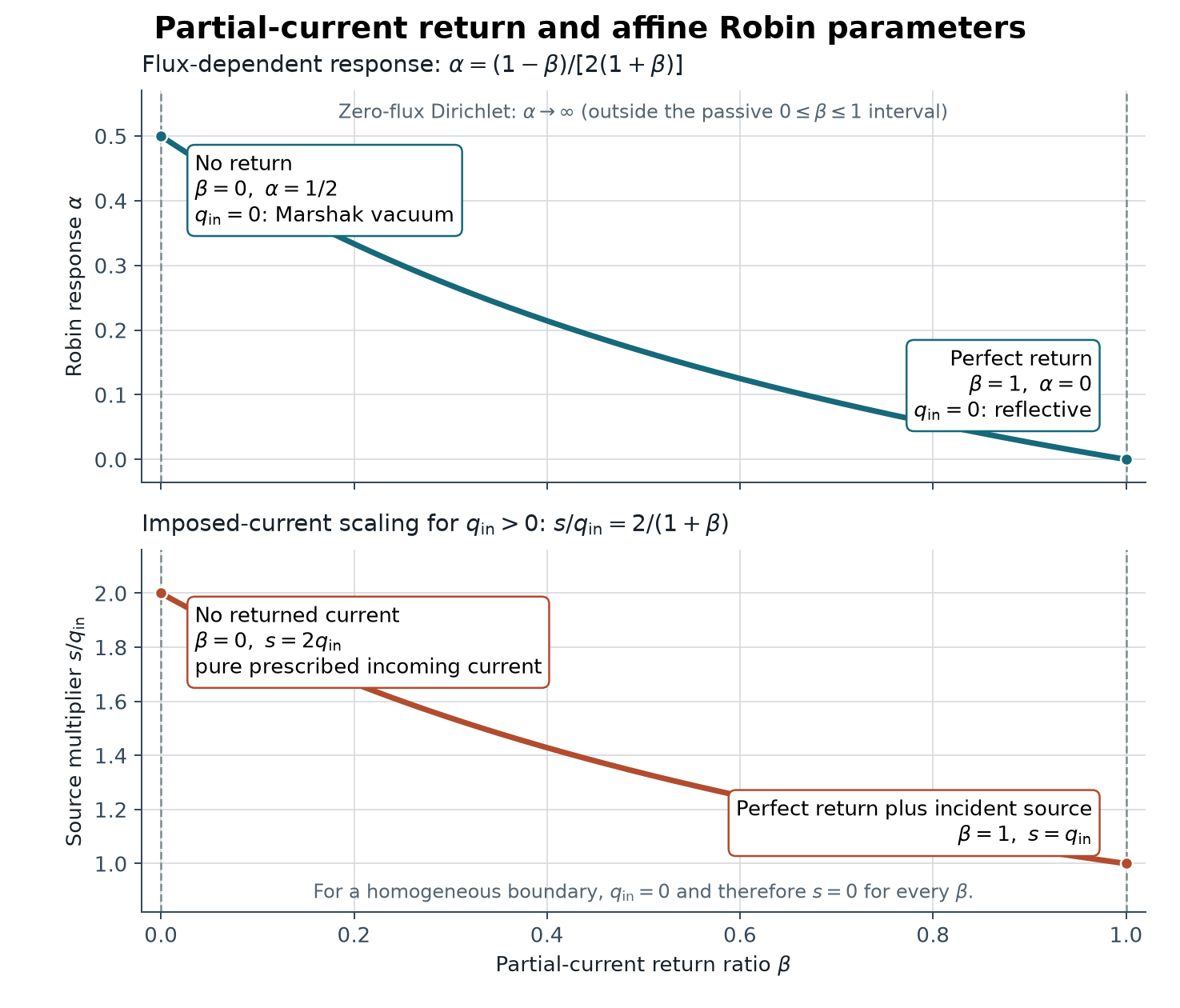
The upper panel shows how the passive partial-current return ratio \(\beta\) maps to the flux-dependent Robin response \(\alpha\). The lower panel shows the normalized imposed-current term for \(q_{\mathrm{in}}>0\); when \(q_{\mathrm{in}}=0\), \(s=0\) for every \(\beta\). The endpoint labels therefore distinguish the homogeneous Marshak-vacuum and reflective limits from their affine counterparts with an independent incident source. Zero-flux Dirichlet is the separate limit \(\alpha\rightarrow\infty\) and does not lie on the passive \(0\leq\beta\leq1\) curve.

Combining the affine Robin condition with the one-sided finite-volume approximation gives

\[ \begin{aligned} \phi_b &= \frac{D_c\phi_c+sd}{D_c+\alpha d}, \\ J_{\mathrm{out}} &= \frac{\alpha D_c}{D_c+\alpha d}\phi_c - \frac{sD_c}{D_c+\alpha d}. \end{aligned} \]

In the finite-volume operator, the first term contributes the Robin conductance

\[ \mathcal{G}_{cf}=\frac{\alpha D_cA_f}{D_c+\alpha d} \]

to the matrix diagonal, and the incoming term contributes

\[ b_{\partial,cf}=\frac{sD_cA_f}{D_c+\alpha d} \]

to the boundary right-hand side. For \(\alpha=0\), Morana evaluates this as \(b_{\partial,cf}=sA_f\), including when \(D_c=0\): a perfectly returning boundary with an imposed incident current has a prescribed inward net current and no flux-dependent loss term.

For \(D_c=0\) and \(\alpha>0\), both the conductance and additive source are zero. Dirichlet conductance is also zero when \(D_c=0\). These are the implementation’s zero-diffusion conventions; the face-flux formulas that divide by \(D_c+\alpha d\) do not define a face flux when both \(D_c\) and \(\alpha\) vanish.

Setting \(\beta=0\) removes the returned-current component; allowing nonzero \(\beta\) combines returned outgoing current with the independent incident source through the same affine assembly path. The surface-averaged partial current \(q_{\mathrm{in}}\) has units \(\mathrm{n\,cm^{-2}\,s^{-1}}\).

Prescribed nonzero Dirichlet data remain a distinct face-flux condition.

Albedo convention

Morana’s \(\beta\) is a scalar P1 partial-current return ratio. It is not generally equivalent to a quantity called albedo in a transport code. For example, OpenMC’s Surface.albedo scales particle weight at reflective, periodic, or white surface interactions, and OpenMC distinguishes specular reflective behavior from diffuse white behavior in its boundary-condition guide. Interpreting that value as Morana’s \(\beta\) is an explicit diffusion approximation and does not preserve the transport model’s angular distinction. Any comparison or conversion must identify the albedo convention being used.

Solver acceptance and balances

Norms

Morana uses two discrete \(L^2\) norms. For any packed node/group vector \(\mathbf x\),

\[ \lVert\mathbf x\rVert_2^2=\sum_{n,g}x_{n,g}^2, \qquad \lVert\mathbf x\rVert_V^2=\sum_{n,g}V_nx_{n,g}^2. \]

The Euclidean norm \(\lVert\cdot\rVert_2\) measures algebraic equation defects in both solve modes. The volume-weighted norm \(\lVert\cdot\rVert_V\) compares successive physical flux shapes, weighting each cell by its volume.

Linear algebra execution

The fixed-source system uses \(B=A-F\) and right-hand side \(\mathbf b\). An ordinary criticality inner iteration uses \(B=A\) and right-hand side \(F\boldsymbol\phi^{(n)}\); a fixed-Wielandt iteration changes \(B\) as defined below. Morana offers either a sparse direct reference solve or restarted GMRES from the zero initial guess. Both policies solve the same algebraic problem with the same physical-flux acceptance criteria.

For GMRES with a preconditioner \(P\), the iterated system is the left-preconditioned form

\[ P^{-1}B\mathbf x=P^{-1}\mathbf b. \]

NoPreconditioner sets \(P=I\). JacobiPreconditioner uses the finite, nonzero diagonal of \(B\) as \(P\). IluPreconditioner uses a threshold incomplete-LU factorization of \(B\) with the configured drop tolerance and fill bound as \(P\). These choices change GMRES’s Krylov iteration, not the system \(B\mathbf x=\mathbf b\) or the accepted physical flux. The GMRES and preconditioner constructions are described by Barrett et al. (1994).

Morana uses SciPy’s left-preconditioned GMRES implementation. It minimizes a preconditioned residual, whereas SciPy tests its own termination criterion against the original residual (SciPy GMRES documentation).

Morana independently applies its own symmetric true-relative-residual check to every direct or GMRES candidate,

\[ r_{\mathrm{lin}}(B,\mathbf x,\mathbf b)= \frac{\lVert\mathbf b-B\mathbf x\rVert_2} {\lVert\mathbf b\rVert_2+\lVert B\mathbf x\rVert_2}. \]

When both actions are zero, Morana defines this residual as zero. The check uses the candidate after admissible negative roundoff has been set to zero. Thus a backend success status or a small preconditioned residual alone cannot accept a result. The modeling and solver workflow defines the per-solve setup and reuse lifetime for those numerical resources.

Balance terms

The reported net_scattering term combines signed scattering-neutron coupling with the ordinary outscatter already included in removal. Its domain-total value for group \(g\) is

\[ \begin{aligned} \mathrm{net\ scattering}_g ={}& \sum_{n,h} C_{h,g,n}V_n\phi_{h,n} \\ &- \sum_n\bigl(\Sigma_{r,g,n}-\Sigma_{a,g,n}\bigr) V_n\phi_{g,n}. \end{aligned} \]

The first line is reported separately as scattering_coupling; the second is the ordinary event-loss portion of removal. With unit multiplicity, net_scattering cancels after summing over all groups, although its individual group values need not vanish. With non-unit multiplicity, the domain-wide sum retains the corresponding neutron gain or loss. The solve-mode sections below combine this term with fission, source, absorption, and leakage diagnostics.

Fixed-source residual and balance

For a solution of the canonical fixed-source system, the symmetrically normalized Euclidean equation residual is

\[ r_{\mathrm{fixed}}= \frac{\lVert\mathbf b-(A-F)\boldsymbol{\phi}\rVert_2} {\lVert\mathbf b\rVert_2+\lVert(A-F)\boldsymbol{\phi}\rVert_2}. \]

Using the source functionals defined above, a groupwise balance distinguishes production \(P_g(\boldsymbol\phi)\) by incident group from emission \(E_g(\boldsymbol\phi)\) into an outgoing group. Their sums agree, but their individual group values need not. At convergence, the fixed-source group balance is

\[ \begin{aligned} \mathrm{source}_g+\mathrm{boundary\ source}_g +E_g(\boldsymbol\phi)+\mathrm{net\ scattering}_g -\mathrm{absorption}_g-\mathrm{radial\ leakage}_g -\mathrm{axial\ leakage}_g=0. \end{aligned} \]

For prescribed nonzero Dirichlet flux or incoming current, \(\mathbf b_\partial\) supplies the explicit boundary_source term. The reported leakage terms contain the flux-dependent conductance losses; subtract boundary_source from their sum to obtain net outward leakage for inhomogeneous boundaries. Internal-face currents cancel in the domain total. Axial currents cancel across active-to-active layer interfaces in that global balance; only exposed axial-face loss remains. A layer-resolved balance retains the signed axial contribution before this global contraction.

k-effective iteration and balance

The k-effective solve uses the canonical multiplication eigenproblem defined under Multigroup formulation. It has no independent volumetric or boundary source and requires a homogeneous condition on every exposed hex-z face, positive fission production, and a nonsingular assembled loss matrix \(A\). Morana’s three-part convergence criterion, iterate admissibility checks, and final physical normalization are defined below.

The ordinary iteration is the classical power method applied to the implicit operator \(A^{-1}F\) (Gu, 2000). Starting from an all-positive node-major shape normalized to \(P(\boldsymbol{\phi}^{(0)})=1\), the ordinary policy is

\[ \begin{aligned} \mathbf e^{(n)} &= F\boldsymbol{\phi}^{(n)}, \\ A\tilde{\boldsymbol{\phi}}^{(n+1)} &= \mathbf e^{(n)}, \\ k_{\mathrm{eff}}^{(n+1)} &= P\left(\tilde{\boldsymbol{\phi}}^{(n+1)}\right), \\ \boldsymbol{\phi}^{(n+1)} &= \frac{\tilde{\boldsymbol{\phi}}^{(n+1)}} {k_{\mathrm{eff}}^{(n+1)}}. \end{aligned} \]

Fixed Wielandt shift

The convergence of ordinary power iteration is controlled by its modal separation: a subdominant mode near the dominant mode makes its source shape change slowly. A Wielandt shift modifies the inner operator while preserving the physical eigenproblem. For reactor-physics background, including the dominance-ratio motivation and the tradeoff between acceleration and the conditioning of a shifted system, see the open MPACT theory manual (Larsen et al., 2019). The equations below define Morana’s parameterization and normalization convention.

Morana uses one fixed, nonnegative inverse-multiplication-factor shift \(\sigma\). With the same production-normalized previous shape, it solves

\[ \left(A-\sigma F\right)\mathbf u^{(n+1)} =F\boldsymbol\phi^{(n)}, \]

then recovers the physical multiplication factor and normalizes the next shape as

\[ q^{(n+1)}=P\left(\mathbf u^{(n+1)}\right), \qquad k_{\mathrm{eff}}^{(n+1)}= \left(\sigma+\frac{1}{q^{(n+1)}}\right)^{-1}, \qquad \boldsymbol\phi^{(n+1)}= \frac{\mathbf u^{(n+1)}}{q^{(n+1)}}. \]

To see the useful shift range, write the generalized eigenvalues as \(A\boldsymbol\phi_i=\mu_iF\boldsymbol\phi_i\), where the physical fundamental mode has the smallest positive inverse multiplication factor \(\mu_1=1/k_{\mathrm{eff}}\). The iteration operator \((A-\sigma F)^{-1}F\) has eigenvalues \(1/(\mu_i-\sigma)\) for these modes. For a real positive spectrum ordered \(\mu_1<\mu_2\leq\cdots\), \(0\leq\sigma<\mu_1\) keeps the fundamental transformed eigenvalue positive and dominant. Moving \(\sigma\) toward \(\mu_1\) improves its separation from the other modes and accelerates the outer iteration. At the limit the shifted operator is singular. A shift above it can lose inverse positivity and produce nonphysical negative flux, while a shift too close below it makes the inner linear system poorly conditioned.

Setting \(\sigma=0\) recovers the ordinary iteration above. WielandtShiftSettings holds one constant shift for the entire solve. A usable value normally comes from a reference calculation and must leave the shifted operator solvable and the recovered inverse multiplication factor positive; an unusable value raises an error. The inner linear residual is evaluated for the selected ordinary or shifted system, while the outer residual always evaluates the original, unshifted eigenvalue equation. Criticality convergence therefore depends on the outer criteria as well as the shifted linear solves.

Every inner-solve candidate must be finite and numerically nonnegative. Negative components within the roundoff tolerance are cleaned to zero; a significantly negative component, nonpositive production, failed inner solve, or nonfinite iterate rejects the solve. Zero components are valid, and a reducible system need not have a unique dominant shape.

Convergence requires all three measures:

\[ \delta_{k_{\mathrm{eff}}} =\frac{|k_{\mathrm{eff}}^{(n+1)}-k_{\mathrm{eff}}^{(n)}|} {|k_{\mathrm{eff}}^{(n+1)}|}, \qquad \delta_\phi= \frac{\lVert\boldsymbol{\phi}^{(n+1)}-\boldsymbol{\phi}^{(n)}\rVert_V} {\lVert\boldsymbol{\phi}^{(n+1)}\rVert_V}, \]

where the common volume-weighted norm \(\lVert\cdot\rVert_V\) compares flux shape. The symmetric Euclidean equation residual is

\[ r_{k_{\mathrm{eff}}}= \frac{\left\lVert F\boldsymbol{\phi}^{(n+1)} /k_{\mathrm{eff}}^{(n+1)} -A\boldsymbol{\phi}^{(n+1)}\right\rVert_2} {\left\lVert F\boldsymbol{\phi}^{(n+1)} /k_{\mathrm{eff}}^{(n+1)}\right\rVert_2 +\left\lVert A\boldsymbol{\phi}^{(n+1)}\right\rVert_2}. \]

Only after convergence is the unit-production shape scaled to the requested physical normalization. FissionSourceNormalization specifies a fission source rate in \(\mathrm{n\,s^{-1}}\), so the scaled flux satisfies \(\sum_g P_g(\boldsymbol\phi)=\mathrm{fission\ source\ rate}\). For PowerNormalization, each fissionable material provides a groupwise recoverable-energy production cross section \(\kappa\Sigma_{f,g}\) in \(\mathrm{eV\,cm^{-1}}\). After conversion to joules, the final scale satisfies

\[ \sum_n V_n\sum_g \kappa\Sigma_{f,g,n}\phi_{g,n} = \mathrm{requested\ power}\quad [\mathrm{W}]. \]

Morana verifies this requirement for every active fissionable material before assembling the finite-volume criticality operators; it never forms a partial power response from only the materials that supplied energy data.

Power normalization uses this input directly because neutron-production data alone do not determine the recoverable energy released per fission. The destination-group eigenvalue source is \(K_g(\boldsymbol\phi,k_{\mathrm{eff}})\) as defined above.

The groupwise criticality balance distinguishes incident-group fission production \(P_g(\boldsymbol\phi)\) from outgoing-group eigenvalue source \(K_g(\boldsymbol\phi,k_{\mathrm{eff}})\). With absorption, radial and axial leakage, and signed scattering-neutron coupling, the group equation closes as

\[ K_g(\boldsymbol\phi,k_{\mathrm{eff}}) -\mathrm{absorption}_g-\mathrm{radial\ leakage}_g -\mathrm{axial\ leakage}_g+\mathrm{net\ scattering}_g=0. \]

With unit scattering multiplicity, summing this equation over groups cancels net_scattering. With non-unit multiplicity, that term instead retains the associated neutron gain or loss. The remaining source and loss terms have units \(\mathrm{n\,s^{-1}}\).

References

Barrett et al. (1994). R. Barrett, M. Berry, T. F. Chan, J. Demmel, J. Donato, J. Dongarra, V. Eijkhout, R. Pozo, C. Romine, and H. van der Vorst, Templates for the Solution of Linear Systems: Building Blocks for Iterative Methods, 2nd edition, SIAM, 1994. Open online sections: 2.3.4, “Generalized Minimal Residual (GMRES)”; 3.1.2, “Left and right preconditioning”; 3.2, “Jacobi Preconditioning”; and 3.4, “Incomplete Factorization Preconditioners”.

Bell and Glasstone (1970). G. I. Bell and S. Glasstone, Nuclear Reactor Theory, TID-25606, U.S. Atomic Energy Commission, 1970. OSTI bibliographic record and open full text.

Boyd et al. (2019). W. Boyd, A. Nelson, P. K. Romano, S. Shaner, B. Forget, and K. Smith, “Multigroup Cross-Section Generation with the OpenMC Monte Carlo Particle Transport Code,” Nuclear Technology, 205(7), 928–944, 2019, DOI 10.1080/00295450.2019.1571828. Open full text.

Eymard, Gallouët, and Herbin (2000). R. Eymard, T. Gallouët, and R. Herbin, “Finite Volume Methods,” in Handbook of Numerical Analysis, volume 7, pp. 713–1020, 2000, DOI 10.1016/S1570-8659(00)07005-8. Open author manuscript and HAL record.

Gu (2000). M. Gu, “Power Method” (Section 4.3.1), in Z. Bai, J. Demmel, J. Dongarra, A. Ruhe, and H. van der Vorst, editors, Templates for the Solution of Algebraic Eigenvalue Problems: A Practical Guide, SIAM, Philadelphia, 2000. Open online section.

Larsen et al. (2019). E. W. Larsen, B. S. Collins, B. A. Kochunas, and S. R. Stimpson, editors, MPACT Theory Manual, version 4.1, CASL-U-2019-1874-001, Consortium for Advanced Simulation of LWRs, 2019. Open full text, Section 7.7 “CMFD Eigenvalue Solvers”.

Ványi et al. (2021). A. S. Ványi, M. Hursin, and S. Czifrus, “Investigation of Recently Introduced Diffusion Coefficient Generation Methods,” in Proceedings of the 30th International Conference Nuclear Energy for New Europe, Bled, Slovenia, September 6–9, 2021, paper 311. Open full text.