One-dimensional axial core-reflector case

examples/one_group_keff.py is a one-group criticality verification case with an analytic two-region axial diffusion solution. It uses one planar hexagon and reflective lateral faces, so no radial leakage is present and the hex-z model reduces exactly to a one-dimensional problem in \(z\). The fixed 120-layer discretization is compared with the analytic multiplication factor and source-normalized cell-average flux.

The lower part of the column is a fissionable core, and the upper part is a nonfissioning reflector. The bottom is reflective and the reflector top has Morana’s Marshak-vacuum condition. The example writes axial_flux_comparison.png and a material-aware result.vtm under artifacts/examples/one_group_keff/ by default.

Model

The core occupies \(0\le z\le H_c\) and the reflector occupies \(H_c\le z\le H_c+H_r\), where

\[ H_c=100\ \mathrm{cm}, \qquad H_r=50\ \mathrm{cm}. \]

The one-group material data are:

Region	\(D\) [cm]	\(\Sigma_a\) [cm\(^{-1}\)]	\(\nu\Sigma_f\) [cm\(^{-1}\)]
Core	1.20	0.010	0.012
Reflector	1.50	0.002	0

The example explicitly supplies sigma_s=[[0.0]]. A center-only HexPlanarMesh has one active cell in every axial layer. The radial faces and physical bottom face are reflective, while the physical top face is vacuum. The calculation uses 80 equal core layers and 40 equal reflector layers, each \(1.25\ \mathrm{cm}\) high. The horizontal hex area multiplies every term in the one-dimensional balance and does not alter the continuous eigenvalue or flux shape.

Analytic eigenpair

The one-group criticality equation in the core is

\[ -D_c\frac{d^2\phi_c}{dz^2}+\Sigma_{a,c}\phi_c =\frac{\nu\Sigma_{f,c}}{k_{\mathrm{eff}}}\phi_c. \]

Define the positive fundamental-mode buckling and reflector decay constant as

\[ B^2= \frac{\nu\Sigma_{f,c}/k_{\mathrm{eff}}-\Sigma_{a,c}}{D_c}, \qquad \kappa^2=\frac{\Sigma_{a,r}}{D_r}. \]

The reflective bottom condition \(d\phi_c/dz=0\) at \(z=0\) gives the core shape with unit amplitude

\[ \phi_c(z)=\cos(Bz). \]

Let \(s=H_c+H_r-z\) be distance downward from the physical top. Morana’s vacuum preset is the homogeneous current condition

\[ J_{\mathrm{out}}=-D_r\frac{d\phi_r}{dz}=\frac12\phi_r \qquad\text{at }s=0. \]

Consequently, the reflector shape that already satisfies the top condition is

\[ \phi_r(z)=C\left[ \cosh(\kappa s)+a\sinh(\kappa s) \right], \qquad a=\frac{1}{2D_r\kappa}. \]

Flux and upward normal current are continuous at the material interface; the flux derivative changes with the diffusion coefficient. Eliminating \(C\) gives one scalar equation for the fundamental root \(0<B<\pi/(2H_c)\):

\[ D_cB\tan(BH_c) =D_r\kappa \frac{\sinh(\kappa H_r)+a\cosh(\kappa H_r)} {\cosh(\kappa H_r)+a\sinh(\kappa H_r)}. \]

An independent bracketed scalar root finder gives

\[ B=0.01303438162\ \mathrm{cm}^{-1}, \qquad k_{\mathrm{eff}} =\frac{\nu\Sigma_{f,c}}{\Sigma_{a,c}+D_cB^2} =1.1760239153, \]

and flux continuity determines \(C\). This reference calculation is independent of Morana’s operators and solver.

Discrete comparison

An eigenfunction has arbitrary amplitude. Both solutions are normalized to the configured fission production \(P^\star=10^{15}\ \mathrm{n\,s^{-1}}\). For a single planar-cell area \(A_{\mathrm{hex}}\), the analytic scale factor is chosen so that

\[ P^\star=A_{\mathrm{hex}}\nu\Sigma_{f,c} \int_0^{H_c}\phi_c(z)\,dz. \]

Morana stores a cell-average scalar flux, so the reference for each axial layer \([z_i,z_{i+1}]\) is the exact average

\[ \bar\phi_i=\frac{1}{z_{i+1}-z_i} \int_{z_i}^{z_{i+1}}\phi(z)\,dz. \]

The plot below overlays the smooth analytic flux, Morana’s cell averages, and the analytic cell averages. It also marks the core-reflector interface.

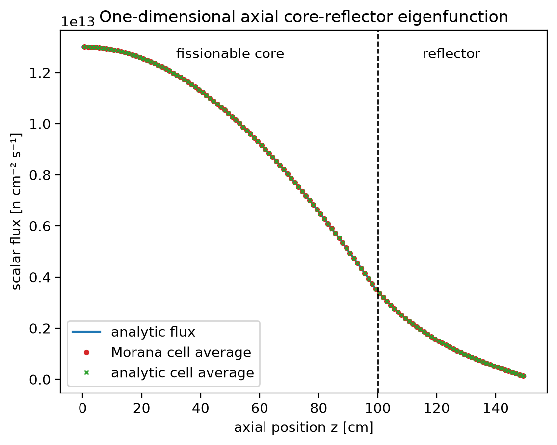
For the discretization of 80 core and 40 reflector layers, the numerical comparison is:

Quantity	Analytic reference	Morana result	Relative difference
\(k_{\mathrm{eff}}\)	1.1760239153	1.1760264857	\(2.186\times10^{-6}\)
Source-normalized axial cell-average flux	–	–	\(3.735\times10^{-5}\) relative L2

The flux measure is the ordinary L2 norm of the 120 compared cell-average values. All layers have the same height and planar area, so it is also the volume-weighted relative L2 norm for this particular mesh. The remaining difference is the finite-volume discretization error, including the discrete core-reflector interface and vacuum-face closures.

Run it

From the repository root with Morana installed in the active environment:

python examples/one_group_keff.py

Pass --output-dir PATH to write the PNG and VTM files elsewhere. See the maintained examples guide for the complete runnable-example list, theory and numerical conventions for Morana’s finite-volume and boundary equations, and the verification overview for the scope of the comparison.

To regenerate the checked-in figure on this page, run:

python examples/one_group_keff.py --documentation-assets-dir docs/assets